A graded lexicographic index, part 1

This post is going to introduce a way to index elements of the bucketspace

This is basically equivalent to indexing the ways you can put indistinguishable balls into distinguishable buckets, hence the name.

Why is this useful? There are a number of pretty good reasons. For one thing, such an index is the key to providing a total ordering of that is a graded lexicographic ordering (i.e., something akin to a dictionary ordering in which words of length 1 appear first in order, then words of length 2, and so on) which can probably be used in lots of places (it seems like the sort of thing that could be a 35-40 rated exercise in Knuth depending on hints). A more specific application derives from the fact that multivariate Lagrange interpolation is about as nice as it can possibly be on which is probably why it turned out that Carl de Boor of spline fame anticipated a lot of our early work from 2001 discussed in this post two years beforehand.

But the reason we’re talking about it here is that random walks on have been used as a way of describing network traffic in a past approach by DoD that we’ve drawn a lot of lessons from (the basic idea for translating network packets to random walks was similar to the approach described at the end of a previous post, except that the finite space is used instead of the infinite root lattice ), and we seriously considered running with this framework in tandem with the one that we followed through with.

There are also some cute martingale results that derive from looking at as the configuration space of states for a classical Bose gas and looking at the energy fluctuations of the gas. In fact this line of thinking led in a very circuitous way to the development of a lattice gauge theory for random walks that we’re working on in the hope that it could lead to descriptors generalizing electric and magnetic charges, fields, etc. for dealing with correlations within network traffic–but talking about that more would take us way too far afield, especially since that stuff is still in the research stage.

Getting back on topic, pictures of the graded lex ordering obtained by projecting onto give a little more insight. For example, with and , there are elements or states, and they are ordered as

(0,0,12), (0,1,11), …, (0,12,0), [13 states]

(1,0,11), (1,1,10), …, (1,11,0), [12 states]

(2,0,10), (2,1,9), …, (2,10,0), [11 states]

…

(11,0,1), (11,1,0), [2 states]

(12,0,0). [1 state]

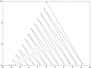
If we just project these points into two dimensions and literally connect the dots in order (except for joining the last point to the first one) we get a pretty clear picture of what’s going on:

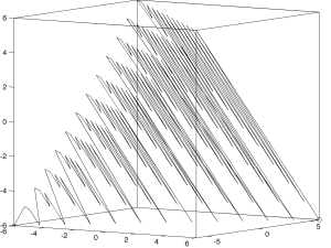
The pattern becomes more obvious if we add a dimension:

It looks recursive, and it is. Since you can read about an essentially equivalent construction in de Boor’s 1999 paper, I won’t belabor the details, though our MATLAB code is different from his and appears to be more fully developed in many respects.

First, here’s how to produce :

function y=lookup(B,b);

% Generates a lookup table with B buckets and b balls.

P1 = pascal(max(b+1,B+1));
P = P1(1:B,:);

numstates = P(B,:);
% ith element gives number of states for B buckets and (i-1) balls

% addermat is a matrix of "row adder" vectors:
addermat = fliplr(eye(B));

%init
look = zeros(1,B);

% Put C = max(c)...the number of balls is b = C-1, so b-1 = C-2
for c = 1:b
 for k = 1:B
 blocksize(c,k) = nchoosek(c+k-2,c-1);
 temp = blocksize(c,k);
 cellblock{k} = look(1:temp,:)+repmat(addermat(k,:),[temp 1]);
 end
 look = cat(1,cellblock{:});
end

y = look;

Next, here’s a recursive index:

function y = stateindex(state)

% B: number of buckets
% b: number of balls

B = length(state);
b = sum(state);

if min(state) < 0 | max(state) > b
 stateindex = 0;  % basic error handling
else
 P1 = pascal(max(b+1,B+1));
 P = P1(1:B,:);
 PA = cat(1,zeros(1,max(b+1,B+1)),P);

 % addermat is a matrix of "row adder" vectors:
 addermat = fliplr(eye(B));

 blocknum = zeros(1,b);
 numblocknum = zeros(1,b);

 substate = state;
 for i = 1:b
 blocknum(i) = max(find(fliplr(substate)));
 substate = substate-addermat(blocknum(i),:);
 numblocknum(i) = PA(blocknum(i),b+2-i);
 end

 stateindex = sum(numblocknum)+1;
end

y = stateindex;

Unfortunately, recursive code usually looks conceptually elegant but performs terribly. In the next post in this series I’ll discuss some more sophisticated methods for indexing states in and related algorithms that avoid this pitfall.