Birds on a wire and the Ising model

Statistical physics is very good at describing lots of physical systems, but one of the basic tenets underlying our technology is that statistical physics is also a good framework for describing computer network traffic. Lots of recent work by lots of people has focused on applying statistical physics to nontraditional areas: behavioral economics, link analysis (what the physicists abusively call network theory), automobile traffic, etc.

In this post I’m going to talk about a way in which one of the simplest models from statistical physics might inform group dynamics in birds (and probably even people in similar situations). As far as I know, the experiment hasn’t been done–the closest work to it seems to be on flocking (though I’ll give $.50 and a Sprite to the first person to point out a direct reference to this sort of thing). I’ve been kicking it around for years and I think that at varying scopes and levels of complexity, it might constitute anything from a really good high school science fair project to a PhD dissertation. In fact I may decide to run with this idea myself some day, and I hope that anyone else out there who wants to do the same will let me know.

The basic idea is simple. But first let me show you a couple of pictures.

Source: http://www.flickr.com/photos/blmurch/ / CC BY-SA 2.0

Notice how the tree in the picture above looks? There doesn’t seem to be any wind. But I bet that either the birds flocked to the wire together or there was at least a breeze when the picture below was taken:

Source: http://www.flickr.com/photos/paul_garland/ / CC BY-SA 2.0

Because the birds are on wires, they can face in essentially one of two directions. In the first picture it looks very close to a 60%-40% split, with most of the roughly 60 birds facing left. In the second picture, 14 birds are facing right and only one is facing left.

Now let me show you an equation:

If you are a physicist you already know that this is the Hamiltonian for the spin-1/2 Ising model with an applied field, but I will explain this briefly. The Hamiltonian is really just a fancy word for energy. It is the energy of a model (notionally magnetic) system in which spins that occupy sites that are (typically) on a lattice (e.g., a one-dimensional lattice of equally spaced points) take the values and can be taken as caricatures of dipoles. The notation indicates that the first sum is taken over nearest neighbors in the lattice: the spins interact, but only with their neighbors, and the strength of this interaction is reflected in the exchange energy The strength of the spins’ interaction with an applied (again notionally magnetic) field is governed by the field strength This is the archetype of spin models in statistical physics, and it won’t serve much for me to reproduce a discussion that can be found many other places (you may like to refer to Goldenfeld’s Lectures on Phase Transitions and the Renormalization Group, which also covers the the renormalization group method that inspires the data reduction techniques used in our software). Suffice it to say that these sorts of models comprise a vast field of study and already have an enormous number of applications in lots of different areas.

Now let me talk about what the pictures and the model have in common. The (local or global) average spin is called the magnetization. Ignoring an arbitrary sign, in the first picture the magnetization is roughly 0.2, and in the second it’s about 0.87. The 1D spin-1/2 Ising model is famous for exhibiting a simple phase transition in magnetization: indeed, the expected value of the magnetization for in the thermodynamic limit is shown in every introductory statistical physics course worth the name to be

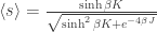
where is the inverse temperature (in natural units). As ever, a picture is worth a thousand words:

For and it’s easy to see that But if and , then taking the subsequent limit yields a magnetization of At zero temperature the model becomes completely magnetized–i.e., totally ordered. (Finite-temperature phase transitions in magnetization in the real world are of paramount importance for superconductivity.)

And at long last, here’s the point. I am willing to bet ($.50 and a Sprite, as usual) that the arrangement of birds on wires can be well described by a simple spin model, and probably the spin-1/2 Ising model provided that the spacing between birds isn’t too wide. I expect that the same model with varying parameters works for many–or even most or all–species in some regime, which is a bet on a particularly strong kind of universality. Neglecting spacing between birds, I expect the effective exchange strength to depend on the species of bird, and the effective applied field to depend on the wind speed and angle, and possibly the sun’s relative location (and probably a transient to model the effects of arriving on the wire in a flock). I don’t have any firm suspicions on what might govern an effective temperature here, but I wouldn’t be surprised to see something that could be well described by Kawasaki or Glauber dynamics for spin flips: that is, I reckon that–as usual–it’s necessary to take timescales into account in order to unambiguously assign a formal or effective temperature (if the birds effectively stay still, then dynamics aren’t relevant and the temperature should be regarded as being already accounted for in the exchange and field parameters). I used to think about doing this kind of experiment using tagged photographs or their ilk near windsocks or something similar, but I can’t see how to get any decent results that way without more effort than a direct experiment. I think it probably ought to be done (at least initially) in a controlled environment.

Anyways, there it is. The experiment always wins, but I have a hunch how it would turn out.

UPDATE 30 Jan 2010: Somebody had another interesting idea involving birds on wires.